Table Of Content
Finally, the researchers asked participants to rate their current level of disgust and other emotions. The primary results of this study were that participants in the messy room were in fact more disgusted and made harsher moral judgments than participants in the clean room—but only if they scored relatively high in private body consciousness. Experimentwise error may be more of a problem in factorial designs than in RCTs because multiple main and interactive effects are typically examined. In a 5-factor experiment there are 31 main and interaction effects for a single outcome variable, and more if an outcome is measured at repeated time points and analyzed in a longitudinal model with additional time effects.

Understanding Variable Effects in Factorial Designs
This paper will use smoking treatment research to illustrate its points, but its content is broadly relevant to the development and evaluation of other types of clinical interventions. Also, it will focus primarily on research design and design implementation rather than on statistical analysis (for relevent discussion of statistical analysis see Box, Hunter, & Hunter, 2005; Keppel, 1991). Factorial experiments can be used when there are more than two levels of each factor. However, the number of experimental runs required for three-level (or more) factorial designs will be considerably greater than for their two-level counterparts. Factorial designs are therefore less attractive if a researcher wishes to consider more than two levels.
Sums of Squares
In many cases, though, the factor levels are simply categories, and the coding of levels is somewhat arbitrary. For example, the levels of an 6-level factor might simply be denoted 1, 2, ..., 6. Physiological measures involve measuring participants’ physiological responses, such as heart rate, blood pressure, or brain activity, using specialized equipment. These measures may be invasive or non-invasive, and may be administered in a laboratory or clinical setting. This involves dividing participants into subgroups or blocks based on specific characteristics, such as age or gender, in order to reduce the risk of confounding variables. This design involves randomly assigning participants to one of two or more treatment groups, with each group receiving one treatment during the first phase of the study and then switching to a different treatment during the second phase.
Exploring hydrothermal liquefaction (HTL) of digested sewage sludge (DSS) at 5.3 L and 0.025 L bench scale using ... - Nature.com
Exploring hydrothermal liquefaction (HTL) of digested sewage sludge (DSS) at 5.3 L and 0.025 L bench scale using ....
Posted: Wed, 01 Nov 2023 07:00:00 GMT [source]
Checking Residuals Using Minitab's Four in One Plot
One independent variable was disgust, which the researchers manipulated by testing participants in a clean room or a messy room. The other was private body consciousness, a participant variable which the researchers simply measured. Another example is a study by Halle Brown and colleagues in which participants were exposed to several words that they were later asked to recall (Brown, Kosslyn, Delamater, Fama, & Barsky, 1999)[1]. Some were negative health-related words (e.g., tumor, coronary), and others were not health related (e.g., election, geometry). The non-manipulated independent variable was whether participants were high or low in hypochondriasis (excessive concern with ordinary bodily symptoms).
Interaction Effects
Moreover, if instead of “off” or no-treatment conditions, less intensive levels of components are used, then even more ICs must be delivered (albeit some of reduced intensity). In Chapter 1 we briefly described a study conducted by Simone Schnall and her colleagues, in which they found that washing one’s hands leads people to view moral transgressions as less wrong [SBH08]. In a different but related study, Schnall and her colleagues investigated whether feeling physically disgusted causes people to make harsher moral judgments [SHCJ08]. In this experiment, they manipulated participants’ feelings of disgust by testing them in either a clean room or a messy room that contained dirty dishes, an overflowing wastebasket, and a chewed-up pen. They also used a self-report questionnaire to measure the amount of attention that people pay to their own bodily sensations. They also measured some other dependent variables, including participants’ willingness to eat at a new restaurant.
Basic Elements of RCT and Factorial Designs
This is what was seen graphically, since the graph with dosage on the horizontal axis has a slope with larger magnitude than the graph with age on the horizontal axis. In the previous section, we looked at a qualitative approach to determining the effects of different factors using factorial design. Now we are going to shift gears and look at factorial design in a quantitative approach in order to determine how much influence the factors in an experiment have on the outcome. A main effects situation is when there exists a consistent trend among the different levels of a factor. From the example above, suppose you find that as dosage increases, the percentage of people who suffer from seizures increases as well.
This is a matter of knowing something about the context for your experiment. When choosing the levels of your factors, we only have two options - low and high. You can pick your two levels low and high close together or you can pick them far apart.
In most cases the levels are quantitative, although they don't have to be. Sometimes they are qualitative, such as gender, or two types of variety, brand or process. As we have already seen, researchers conduct correlational studies rather than experiments when they are interested in noncausal relationships or when they are interested variables that cannot be manipulated for practical or ethical reasons. In this section, we look at some approaches to complex correlational research that involve measuring several variables and assessing the relationships among them. As an exercise toward this goal, we will first take a closer look at extracting main effects and interactions from tables.
Notation
The result of this study was that the participants high in hypochondriasis were better than those low in hypochondriasis at recalling the health-related words, but they were no better at recalling the non-health-related words. The other was private body consciousness, a variable which the researchers simply measured. Another example is a study by Halle Brown and colleagues in which participants were exposed to several words that they were later asked to recall [BKD+99]. Some were negative, health-related words (e.g., tumor, coronary), and others were not health related (e.g., election, geometry).
The last four column vectors belong to the A × B interaction, as their entries depend on the values of both factors, and as all four columns are orthogonal to the columns for A and B. Belong to the A × B interaction; interaction is absent (additivity is present) if these expressions equal 0.[13][14] Additivity may be viewed as a kind of parallelism between factors, as illustrated in the Analysis section below. Time series analysis is used to analyze data collected over time in order to identify trends, patterns, or changes in the data. Self-report measures involve asking participants to report their thoughts, feelings, or behaviors using questionnaires, surveys, or interviews.
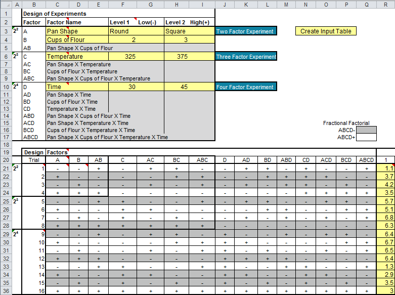
This table reflects the combinations of intervention components (conditions) that is generated by the crossing of two levels of five factors in a factorial design (Schlam et al. 2016). As the factorial design is primarily used for screening variables, only two levels are enough. Often, coding the levels as (1) low/high, (2) -/+, (3) -1/+1, or (4) 0/1 is more convenient and meaningful than the actual level of the factors, especially for the designs and analyses of the factorial experiments.
That is, one should include only those ICs that are thought to be compatible, not competitive. The choice of control conditions can also affect burden and complexity for both staff and patients. In this regard, “off” conditions (connoting a no-treatment control condition as one level of a factor) have certain advantages. They are relatively easy to implement, they do not add burden to the participants, and they should maximize sensitivity to experimental effects (versus a low-treatment control).
For larger numbers, the factor can be considered extremely important and for smaller numbers, the factor can be considered less important. The sign of the number also has a direct correlation to the effect being positive or negative. If the number of combinations in a full factorial design is too high to be logistically feasible, a fractional factorial design may be done, in which some of the possible combinations (usually at least half) are omitted. Experimental design also allows researchers to generalize their findings to the larger population from which the sample was drawn. By randomly selecting participants and using statistical techniques to analyze the data, researchers can make inferences about the larger population with a high degree of confidence. Experimental research design should be used when a researcher wants to establish a cause-and-effect relationship between variables.
For example, people are either low in self-esteem or high in self-esteem; they cannot be tested in both of these conditions. If one of the independent variables had a third level (e.g., using a handheld cell phone, using a hands-free cell phone, and not using a cell phone), then it would be a 3 × 2 factorial design, and there would be six distinct conditions. Notice that the number of possible conditions is the product of the numbers of levels.
This can be seen by noting that the pattern of entries in each A column is the same as the pattern of the first component of "cell". (If necessary, sorting the table on A will show this.) Thus these two vectors belong to the main effect of A. Similarly, the two contrast vectors for B depend only on the level of factor B, namely the second component of "cell", so they belong to the main effect of B. For example, a shrimp aquaculture experiment[9] might have factors temperature at 25° and 35° centigrade, density at 80 or 160 shrimp/40 liters, and salinity at 10%, 25% and 40%.